Tuesday, 25 August 2020

Differences between Weak entity sets and Strong entity sets

Weak entity sets and Strong entity sets


Weak entity sets:


If an entity set do not have sufficient attributes to form a primary key, then such an entity set is termed as a weak entity set. For ex: consider the entity set payment which has the three attributes: payment - number, payment - date and payment -amount.


Payment numbers are typically sequential numbers, starting from 1, generated separately for each loan. Although, each payment entity is distinct, payments for different loans may share the same payment - number. Thus, this entity set does not have a primary key; as such, it is a weak entity set.


In order to be meaningful, weak entity set must be associated with another entity set, called as identifying or owner entity set. This means that a weak entity set is said to be existence dependent on the identifying entity set. An identifying entity set is said to own the weak entity set that it identifies.


The relationship associating the weak entity set with the identifying entity set is called the identifying relationship. Identifying relationship is many to one (M: 1) from the weak entity set to the identifying entity set, and the participation of the weak entity set in the relationship is total.


In our example, the identifying entity set for a payment is loan, and a relationship loan-payment that associates payment entities with their corresponding loan entities is the identifying relationship.


The discriminator of a weak entity set is a set of attributes that allows this distinction to be made. For ex: the discriminator of the weak entity set payment is the attribute payment- number, for each loan, if payment number uniquely identifies one single payment for that loan. A discriminator of a weak entity set is also called the partial key of the entity set.


The primary key of a weak entity set is formed by the primary key of the identifying entity set, plus the weak entity set’s discriminator. In case of the entity set Payment, its primary key (PK) is {loan- number, payment-number}, where Loan - number is the primary key of the identifying entity set, namely loan, and payment - number distinguishes payment entities within the same loan. The identifying relationship set should have no descriptive attributes.

A weak entity set can participate in relationships other than the identifying relationship. For instance, the payment entity could participate in a relationship with the Account entity set, identifying the account from which the payment was made. A weak entity set may participate as owner in an identifying relationship with another weak entity set. It is also possible to have a weak entity set with more than one identifying entity set.


In ER diagrams, a doubly out lined box indicates a weak entity set, and doubly outlined diamond indicates the corresponding identifying relationship.


E-R diagram for weak entity set

Fig: E-R diagram showing weak entity set

In above fig., the weak entity set payment depends on the strong entity set loan via the relationship set loan- payment. The above fig. also depicts the use of double lines to indicate total participation.


The participation of the weak entity set payment in the relationship loan – payment is total, meaning that every payment must be related via loan - payment to some loan. An arrow (🠈) from loan – payment to loan indicates that each payment is for a single loan. The discriminator of a weak entity set is also underlined but with a dashed rather than a solid line.


Strong entity set:


Entity types that consist of key attributes are called strong entity sets. The strong entity set consists of parent entity type or dominant entity type. Strong entity type set can always be represented as complex (composite, multivalued) attributes.


Strong entity set

Here, loan is an entity having a primary key called Loan_no. Hence, loan is a strong entity.


Differences between strong entity set and weak entity set:

Strong entity set

Weak entity set

An entity set having a primary key is termed as strong entity set.

An entity set is termed as weak entity set if its existence depends on other entities i.e. strong entities.

It has sufficient attributes to form a primary key.

A weak entity set does not have sufficient attributes to form a primary key.

Strong entity set is indicated in ER diagrams by a single outlined rectangle.

A weak entity set is indicated in ER diagrams by a doubly outlined rectangle.

The primary key of a strong entity set is formed by primary key of strong entity set.

The primary key of weak entity set is formed by primary key of strong entity set, plus its discriminator.

Strong entity set is not existence dependent on the identifying entity set.

 Weak entity set is said to be existence dependent on the identifying entity set.


Basic Concepts of Entity-Relationship (E-R) Model

Basic Concepts of Entity – Relationship (E – R) Model:

1.    Entity:


An entity can be defined as a ‘thing’ or ‘object’ in the real world that can be distinguished from all other objects. For ex: each person in an organization or enterprise is an entity.


An entity has a set of properties. Furthermore, the values for some set of properties may uniquely identify an entity. For ex: a person may have a Person-ID property, whose value uniquely identifies that person. So, the value 123-456-789 for a Person- ID would uniquely identify one particular person in an organization.


An entity may be concrete such as a person or a book or it may be abstract such as a loan or a holiday or a concept.


2.     Entity set:


An entity set can be defined as a set of entities of the same type that share (have) the same properties or attributes. For ex: the set of all persons who are customers at a given bank can be defined as the entity set Customer.


The individual entities that constitute a set are said to be the extension of the entity set. As such, all the individual bank customers are considered as an extension of the entity set Customer.


Entity sets do not need to be disjoint. For ex: it is possible to define an entity set of all employees of a bank (Employee) and the entity set of all customers of the bank (Customer). A person entity may be an employee entity, a customer entity, both or neither.


3.    Relationship:


A relationship can be defined as an association among several entities. For ex: we can define a relationship that associates customer Vinod with loan L-10. This relationship specifies that Vinod is a customer with a loan number L-10.


4.     Relationship set:


A relationship set is a set of relationships of the same type. Formally, it is a mathematical relation on n>=2 (possibly non distinct entity sets).


What are the various Data Models in DBMS?

 Data Models in DBMS:


A data model is a collection of conceptual tools for describing data - its relationships, semantics and consistency constraints. Data models can be distinguished from one another on the basis of the relationship among data, that is defined and the way the data is conceptually defined.


A primary objective that a data model serves is to evolve a high level data model. It should assist the designer to incorporate a major portion of semantics of database in the schema.


 In DBMS, the data models are broadly classified as:

1.    Object based data models

2.    Record based data models and;

3.    Physical data models


1.    Object Based Data Models:

These models are used in describing data at a logical and view level. They have properties like they provide flexible structure in the capabilities and allow us to specify data constraints explicitly. This model highlights that everything is object having set of attributes.


Examples of data models that fall in this category are:

a)    Entity relationship model

b)    Object oriented model


2.    Record Based Data Models:

The record based data models are used to describe data at a logical and view level. However, they revolve around the records of database and specify the overall structure of database with the help of value of records. This is a key distinguishing factor between the record based and object based model.


These models have got their name record based models because the database is structured in fixed format records of several types. Each record type defines a fixed number of fields or attributes and each field is usually of a fixed length. This results in simple physical level implementations of the database.

Examples of data models that fall in this category are:

a)    Relational model

b)    Network model

c)    Hierarchical model


3.    Physical Data Models:


This model is used to describe data at the lowest level. It actually describes the behaviour of data at disk level. Furthermore, it also describes the way data and data relationships that are maintained while storing them on the disk. As such this leads to the way a DBMS is going to use secondary storage devices for storing and accessing data.


Examples of data models that fall in this category are:

a)    Unifying model

b)    Frame memory model


A.  Network Model:


The data in network model are represented by collection of records. The relationships among data are represented by links, which can be viewed as pointers.

Simply speaking, a pointer is a physical address which identifies where the next record can be found on the disk or we can say that it points to the next address location.


The network model allows each record to have multiple parent and child records forming a lattice structure. Thus, network model supports many to many relationships. The relationship between different records is called sets. This model is used as an easy way of representing objects and their relationships. Following figure shows an example for network database:


Network database

B.  Hierarchical Model:


This model is very similar to network model, as in both the models, the data and relationships among data are represented by using records and links respectively. In this model, records are organized as collection of trees rather than arbitrary graphs.


The data storage is in the form of parent child relationship. An origin of the tree is called the root.  Data that follows the root is called a node and the last node in the series is called as a leaf node. Usually, there is one to many relationship found in this model. Following figure shows an example for hierarchical database:


Hierarchical database

Differences between Relational, Network and Hierarchical Models:


Parameter

Relational model

Network model

Hierarchical model

Relationship

It supports one to many and many to many relationships.

It supports many to many relationships.

It supports one to many relationships.

Nature

It is a table based model, where a table is a collection of rows and columns.

It is based on records and links.

It is based on tree like structure having one root, several nodes and leaf nodes.

Popularity

This model is more popular.

This model is less popular.

This model is less popular.

Applications

It has many applications, almost unlimited.

It is an upgraded version of hierarchical model, so used in the network.

It is mainly used in mainframe and database system.

Data relation

This model uses values to relate data. It does not use pointers or links.

This model uses links to relate data.

This model uses pointers to relate data.


  Storage

The data is stored in the form of tables.

The data is stored in the form of arbitrary graph.

The data is stored in the form of a tree having parent - child relationship.


Monday, 24 August 2020

Operations on Process - Creation, Termination and Concurrent Processes in OS:


Operations on Process:

In most of the operating systems, a processor supports at least two modes of execution:

1.    User mode – it is a less privileged mode. All user programs run in this mode.

2.    Kernel mode – it is a more privileged mode. All the OS related tasks are executed in this mode. A kernel mode is also called as a system mode or control mode.


The mode of execution is indicated by a bit in the program status word (PSW).


1.    Process Creation:


An OS creates a new process with the specified or default attributes and an identifier.  A process may create several new sub-processes.


Syntax for new process creation: CREATE (ProcessID, attributes), where CREATE is a system call. They have two types - Parent process and Child process.


A parent process is a creating process whereas; a child process is created by the parent process. A child process may create another sub processes for which it acts as a parent.  As such, it forms a tree of processes. When OS issues a CREATE system call, it obtains a new PCB from the pool of free memory, fills the fields with parameters (provided and default) and insert the PCB into the ready list. Thus, this makes the specified process eligible for execution.


Commonly required parameters when a process is created include:

·         priority of a process

·         privilege level

·         memory resources

·         access permissions

·         memory protection information, etc.


Moreover, a process will require certain resources such as CPU time, memory, files and IO devices to complete its operation.  When a process creates a sub-process, it may obtain its resources either directly from an OS or it uses the resources of parent process.


When a parent process creates a new child process, they can execute in one of the following way:

1.    Parent continues to execute concurrently with its child.

2.    Parent waits until some or all of its child processes have terminated.


Similarly, with regards to an address space, the two possibilities that can occur:

1.    Child process is a duplicate of the parent process.

2.    Child process has a program loaded into it.


Following are the possible reasons for process creation:

1.    New batch job: a batch job is provided to OS.

2.    Interactive logon: user at a terminal logs on to the system.

3.    Created by OS on behalf of a user program.


2.    Process Termination :


A DELETE system call is used for terminating a process.  A process can terminate itself or it may be terminated by another process using an appropriate system call. When a process is terminated, OS reclaim all the resources that were allocated to it and close all files opened by that process. Further, OS removes PCB and returns it to the free pool. The delete service is a normally invoked as a part of orderly program termination.


Possible reasons for process termination are as follows:

1.    A process has completed its normal operation.

2.    When parent terminates, it terminates the child process.

3.    A process has run longer than the specified total time length.

4.    Process requires more memory than the system can provide.

5.    Process tries to access un-allowed memory location.

6.    An attempt to execute invalid instruction.

7.    Privileged instruction- process tries to use an instruction reserved for OS only.

1.    Protection error - process attempts to use a resource that it is not allowed to use.

2.    If a deadlock exists in the system, an OS may terminate a process.

3.    Data misuse - a piece of data is of wrong type or is not initialised.


Concurrent Processes:


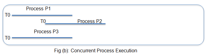
The two processes are said to be serial processes, if the execution of one must complete before the execution of another process starts. The two processes are called concurrent, if they are not serial and their execution can overlap in time. 


Consider the following figure:


Serial process execution


Concurrent process execution


In Fig (a), process P1 starts its execution at time T0; process P2 starts its execution only after process P1 has finished its execution.  Similarly, process P3 starts its execution only after process P2 has finished its execution.  Thus, these processes are said to be serial processes.


Now, consider Fig (b), where the execution time of processes P1, P2 and P3 are overlapped. Therefore, they are called as concurrent processes.


Suspended Processes, Process Control Block (PCB) and Spawning of Processes in OS:


Suspended Processes:

·         They are not immediately available for execution.

·         A process may or may not be waiting for an event.

·         To prevent its execution, a process can be suspended by an OS, parent process, process itself and an agent.

·         A process may not be removed from the suspended state until the agent orders the removal.

·         A technique called swapping is used to move all processes from main memory to disk. When all the processes in the main memory are in blocked state, the OS can suspend one process by putting it in suspended state and transferring it to disk.


 Possible reasons for process suspension are:

1.    Swapping: OS needs to release required main memory to bring in a process that is ready to execute.

2.    Timing: process may go to suspended state while waiting for the next time interval.

3.    Interactive user request: process may be suspended for debugging purposes by user.

4.    Parent process request: to modify the suspended process or to co-ordinate the activity of various descendants of the process.


Process Control Block (PCB):

Every process contains a special data structure called as the process control block. The PCB is used by an operating system for grouping of all information about that particular process. The following figure shows the structure of a PCB:


Process Control Block

1.    Pointer: it points to another process control block. A pointer is used for maintaining the scheduling list.

2.    Process state: process state may be new, ready, running, waiting and so on.

3.    Program counter (PC): it indicates the address of the next instruction to be executed for the current process.

4.    Event information: for a process in the blocked state, this field contains information concerning the event for which the process is waiting.

5.    CPU register: it includes general purpose register, stack pointer (SP), index registers and accumulators (ACC), etc. The total number of registers and type of registers depends upon the computer architecture of a system.

6.    Memory management information: this information may include the values of the base and limit register. It is useful for de-allocating the memory when the process terminates.

7.    Accounting information: this information includes the amount of CPU and real time used, time limits, job or process numbers, account numbers, etc.


A PCB also includes information about CPU scheduling, IO resource management, file management information, process priority, etc. It acts as a repository of information, and this information can vary from a process to process.


When a process is created, hardware registers and flags values are set that are provided by the loader or linker. Whenever that process is suspended, the contents of the processor register are usually saved on the stack and the pointer to the related stack frame is stored in the PCB. So, in this way the hardware state can be restored when the process is scheduled to run again.


Spawning:

A process that creates a new process is named as the parent process, and the created process is called the child process. This method of creating a new process is said to be spawning a process. Furthermore, a child process could itself spawn a new process. This results in formation of tree of processes which provides us hierarchical process structure.


Hierarchical process structure


Concept of a Process in Operating System (OS):

Concept of a Process in OS: 

When an OS runs a program, it is loaded into memory and the control is transferred to the first instruction of that program. After that, the program starts to run. A process can be defined as a program in execution. It is used as a unit of work for a processor. Every process has a program counter (PC), a stack, data section, etc. Furthermore, there can be multiple processes associated with one program. As such, a process is more than a program.


A process consists of components like:

Object program - object program i.e. code to be executed.

Data - data is used for executing the program.

Resources - while executing the program, it may require some resources.

Status - to verify the status of process execution.


The common attributes of a process consists of the hardware state, memory, CPU and the progress (execution status) of that process. Another important consideration is that a program is called a passive entity, while a process is an active entity. A program becomes process when, executable file is loaded into memory.


A process is more than a program code. This program code is generally called as the text section. A data section contains global variables and the heap contains memory that is dynamically allocated during runtime. Whereas, a stack usually has temporary data like temporary variables, local variables, function or subroutine parameters, return addresses, etc. In cases, a same program may have two or more processes that are associated with it. But, they are not considered as separate execution sequences. A program can create multiple processes. For ex: a web browser application.


 Process vs. Programs:


Process vs. Program

Process States:

Whenever a process executes, there occurs change in its state. Usually, a process state is determined by the current activity of the process. Each process may be in one of the following states:


1.    New: the process has just been created.

2.    Running: the process is currently being executed.  A running process has all the resources that are needed for its execution, including the processor.

3.    Waiting: the process is waiting for some event to occur. A running process may become suspended by invoking an IO routine.

4.    Ready: the process is waiting to be assigned to a processor allocated to them by OS so that it can run.

5.    Terminate: the process has finished its execution and no longer requires CPU.


Whenever a process changes its state, an OS updates the process PCB (Process Control Block) in the list that corresponds to its new state. Only one process can be running in any processor at any time. However, there can be many processes in ready and waiting states.  Processes that are in ready state are loaded into a ready queue. A ready queue is a one type of data structure used by an OS to store the processes.


Process states


Transitions of Process States:

New➔Ready:  an OS creates a process and prepares it to be executed. After that OS moves the process into the ready queue.


Ready➔Running: when it is a time to select a process to run, OS selects one of the jobs from the ready queue and move the process from ready state to running state.


Running➔Terminated: when a process completes its execution, then the OS terminates that process from running state. An OS may terminate a process because of some other reasons too. Some possible reasons are time limit exceeded, memory unavailable, access violation, protection error, IO failure, etc.


Running➔Ready: an OS shifts a running process to a ready state when the time slot of the processor expires or it receives an interrupt signal.  Consider an example, suppose process P1 is being executed by processor. Meanwhile, a process P2 generates an interrupt signal to processor. In this case, the processor first compares the priorities of processes P1 and P2.  If P1>P2, then the processor continues the process P1. Otherwise, processor switches to process P2 and the process P1 is moved to the ready state.


Running➔Waiting: if a process requires some event to occur for its completion or if there is an IO device requirement, in such cases a process is put into waiting state. Whenever, an OS cannot not provide IO or that event immediately, a process is moved to waiting state by the OS.


Waiting➔Ready:  a process which is in the blocked state is moved to ready state when the event for which it has been waiting occurs.  For ex: a process is in running state, it need an IO device, then the process moved to blocked or waiting state. Now, when the IO device is provided by OS, the process is moved to ready state from waiting or blocked state.