Friday, 18 September 2020

Shortest Job First (SJF) CPU Scheduling Algorithm


Shortest Job First Scheduling (SJF):

It links with each process the length of the latter’s next CPU burst. When the CPU is free, it is assigned to the process of the ready queue which has smallest next CPU burst. If two processes have the same length, FCFS scheduling is used to break the tie.


SJF scheduling algorithm is used frequently in long term scheduling. This algorithm may be either preemptive or non-preemptive. A preemptive SJF algorithm will preempt the currently executing process, whereas a non- preemptive SJF algorithm will allow the currently running process to finish its CPU burst. Consider the following set of processes with burst time in milliseconds:

Process

Burst time

P1

3

P2

6

P3

4

P4

2

Arrival time of the process is 0 and the processes arrive in the order of P1, P2, P3 and P4. The Gantt chart, waiting time and turnaround time are as follows:


Gantt chart:

SJF Gantt chart


Waiting time:

Process

Waiting time

P1

2

P2

9

P3

5

P4

0


 Turnaround time:

 It is the sum of burst time + waiting time of each process.


Process

Turnaround time

P1

3 + 2 = 5

P2

6 + 9 = 15

P3

4 + 5 = 9

P4

2 + 0 = 2


SJF avg turaround time


SJF algorithm is an optimal algorithm. It gives the minimum average waiting time for a given set of processes. However, SJF algorithm cannot be implemented at the level of short-term CPU scheduling as there is no way to know the length of the next CPU burst. 


First Come First Serve (FCFS) CPU Scheduling Algorithm


CPU Scheduling Algorithms:

These algorithms decide which of the processes in the ready queue is to be allocated the CPU. There are many different CPU scheduling algorithms. Out of these, an algorithm that maximizes CPU utilization and throughput; and minimize turnaround time, waiting time, and response time are considered as best of all algorithms.


First Come First Serve Scheduling (FCFS):


FCFS is the simplest scheduling method. CPU is allocated to the process in the order of arrival. The process that requests the CPU first is allocated the CPU first. FCFS is also called FIFO (First In First Out). FCFS is non - preemptive scheduling algorithm. Implementation of the FCFS policy is easily managed with a FIFO queue.


When a process enters the ready queue, its process control block (PCB) is linked onto the tail of the queue. When the CPU is free, it is allocated to the process at the head of the queue. The running process is removed from the queue.


The performance metric used is average waiting time. Average waiting time for FCFS is often quite long. Usually, FCFS is used in batch systems. Real life analogy of FCFS is buying tickets at the ticket counter. The FCFS is a not suitable for real time systems.


Consider following set of processes that arrive at time 0, with the length of the CPU burst given in milliseconds:


Process

Burst time

P1

24

P2

3

P3

3


Now, we calculate an average waiting time when the processes arrive in the following order:


a)    P1, P2, P3     b)  P2, P3, P1


The Gantt chart for the same is as follows:


For process arrival order,


a)    P1, P2, P3


FCFS Gantt chart-I


Waiting time:


Process

Waiting time

P1

0

P2

24

P3

27


FCFS avg waiting time-I


b)  P2, P3, P1

Gantt chart:

FCFS Gantt chart-II


Waiting time:

Process

Waiting time

P1

6

P2

0

P3

3


FCFS avg waiting time-II

The long CPU burst P1 seriously delays the completion of the shorter bursts P2 and P3.The CPU burst of P1 can be very long and all other processes will have no chance to run at all. It is not responsive. If P2 and P3 are interactive, users won't feel it a reasonable arbitrarily longer than the time really needed. It lengthens the average completion time, since it is possible that all processes completes only after P1 completes.


It reduces IO device utilisation, since all IO bound processes will be waiting long for CPU bound ones. This is called as convoy effect. For these reasons FCFS is usable only when all CPU bursts are known to be short, ex: within the kernel.


 Convoy Effect:

Consider 10 IO bound processes and 1 CPU bound process in the system. IO bound processes pass quickly through the ready queue and suspend them waiting for IO. The CPU bound process arrives at the head of the queue and execute the program until completion. IO bound processes rejoin the ready queue and wait for the CPU bound process releasing the CPU.

IO device is idle until the CPU bound process completes. A convoy effect happens when a set of processes need to use a resource for a short time and one process holds the resource for the long time, blocking all other processes.


Advantages:

·         FCFS is relatively simple to implement.

·         It incurs minimum overhead


Disadvantages:

·         It has unpredictable turnaround time.

·         In FCFS, average waiting time is more.


Performance Metrics or CPU Scheduling Criteria


Scheduling Criteria or Scheduling Methodology:


So many CPU scheduling algorithms are available. Different CPU scheduling algorithms have different properties. In choosing which algorithm to use in a particular situation, we must consider the properties of the various algorithms. The performance metrics are used for the same. We can determine which algorithm is the best algorithm and which one is the worst using the performance metrics.  These performance metrics are as follows:


1. Throughput:


Throughput means how many jobs are completed by the CPU within a time period. If the bigger process, this rate may be a process per hour; for short process throughput might be process per minute.


 2. Turnaround time:

The time interval between the submission of the process and time of the completion is called the turnaround time. Turnaround time is sum of the periods spent waiting to get into memory, waiting in ready queue, executing on the CPU and doing IO.


Turnaround time = waiting time in ready queue + executing time + waiting time in        waiting queue for IO


 3. Waiting time:

 Waiting time is the sum of the periods spent waiting by a process in the ready queue. Generally, a CPU scheduling algorithm having the least average waiting time is said to be the best algorithm. It may be expressed as turnaround time less the actual execution time.


4. Response time:

 Response time is the time duration between the submission and first response. For ex: a process entered in the ready queue at 10:05 a.m., but the process got the first response from the CPU is 10:10 a.m. Then the interval between 10:05 and 10:10 is said to be the response time.


5. CPU utilization:

 This is the percentage of time that the processor is busy. CPU utilization may range from 0 - 100%. In single user systems and real time systems this criteria is less important than the time sharing systems. The load on the system affects the level of utilization that can be achieved. On large and expensive systems, it may be the primary criteria.


6. Priority:

 Give superior treatment to processes having higher priorities.


7. Balanced utilization:

 Apart from CPU utilization, the utilization of other resources like memory, IO devices are also considered.


8. Fairness:

 Avoid the process from starvation. All the processes must be given equal opportunity to execute.

Tuesday, 15 September 2020

3 types of schedulers in OS: Long, short and medium term


 3 Types of Schedulers in OS:


An operating system has many schedulers. There are three main scheduler viz. long term scheduler, short term scheduler, and medium term scheduler.


1. Long Term Scheduler:


It is also termed as job scheduler. Its function is to select the jobs from the pool of jobs (job pool) and load these jobs into main memory (ready queue) of the computer.


The main objective of job scheduler is to provide balanced mix of jobs consisting of IO bound and CPU bound processes. It also controls the degree of multiprogramming. If degree of multiprogramming is stable, then average rate of process creation must be equal to average departure rate of processes leaving the system.

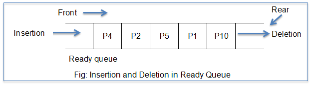
 A ready queue is a nothing but a queue. It is one type of data structure consisting of two ends. One end is called as front and another end is termed as rear. The jobs are loaded into the ready queue through the front; and these jobs are deleted through the rear.


Insertion and deletion in ready queue


A long term scheduler may be absent or minimal in some systems. It is absent in time sharing systems. When a process changes its state from new to ready, long term scheduler comes in play.


2. Short Term Scheduler:


It is also called as CPU scheduler. Function of the short term scheduler is to select a job from the ready queue and gives the control of the CPU to that process with the help of a Dispatcher. The main objective is to increase system performance with respect to the chosen set of criteria. The method of selecting a process from the ready queue depends on the CPU scheduling algorithm. It executes most frequently and is faster compared to long term scheduler.


Dispatcher:


A dispatcher is a module that connects the CPU to the process selected by the short-term scheduler. The main functions of the dispatcher are:

·         switching the CPU from one process to another process (context switch)

·         switching to user mode

·         jumping to the proper location in the user program and ready to start execution


The dispatcher should be fast because it is invoked during each and every process switch. The time taken by dispatcher to stop one process and start another running is known as dispatch latency. The degree of multiprogramming depends greatly on the dispatch latency. It is also sometimes called short term scheduler. If the dispatch latency increases, then degree of multiprogramming decreases.


3. Medium Term Scheduler:


It is a part of swapping function. If a process requests an IO in the middle of the execution, then that process is removed from main memory and loaded into waiting queue. When the IO operation completes, then the job is moved from waiting queue to ready queue. These two operations are commonly termed as swapping and are performed by the medium term scheduler. It reduces the degree of multi programming.


CPU Scheduling concepts in OS: Preemptive and Non-Preemptive


CPU Scheduling:


The CPU scheduling serves as a basis for multi programmed OS. The idea of multiprogramming is simple; if a process or job is waiting for an IO request then the CPU switches from that job to another job. So, the CPU is always kept busy in multiprogramming as it has something to execute at all times. However, in case of a simple computer system, CPU often sits idle until the IO request is granted. Thus, by switching the CPU among processes, an OS can increase productivity and utilization of a computer system.


Scheduling is a fundamental operating system function. Managing the CPU resources is commonly termed as Scheduling. All of the computer resources are scheduled before their use. The CPU is one of the primary resources amongst all resources. Hence, the CPU is also scheduled before use.


An allocation of the CPU to processes is determined using various CPU scheduling algorithms. There are two types of CPU scheduling algorithms:

1.    Non- preemptive scheduling algorithms

2.    Preemptive scheduling algorithms


A CPU has to make scheduling decisions under the following circumstances when a process switches from:

1.    running to waiting state

2.    running to ready state

3.    waiting to ready state or;

4.    when a process terminates.


In non-preemptive scheduling, once the CPU is assigned to a process, the processor do not release until the completion of that process. The CPU will be assigned to some other job only after the previous job has finished. Non – preemptive scheduling takes place for circumstances 1 and 4 mentioned above.  MS Windows 3.1 and Apple’s Mac uses this method of CPU scheduling. It is relatively very simple to implement.


However, in preemptive scheduling, the CPU can release the processes even in the middle of its execution. Consider an example where the CPU is executing process P1. While it is executing, the CPU receives a request signal from process P2.  Then, in this case an OS compares the priorities of processes P1 and P2. If the priority of P1 > P2, then the CPU continues with the execution of process P1. Otherwise, CPU preempts process P1 and assigns it to process P2. Preemptive scheduling takes place for circumstances 2 and 3 mentioned above.


The preemptive scheduling techniques are used to ensure quick response to high priority processes. But, they incur a cost. It is more responsive but it imposes higher overhead because it requires a process switching.


Differences between Preemptive and Non-Preemptive Scheduling:


Preemptive Scheduling

Non-Preemptive Scheduling

It allows a process to be interrupted in the midst of its execution by taking the CPU and allocating it to another process.

It ensures that process gives control of the CPU only when it finishes with its current CPU burst.

It incurs cost associated with access to shared data.

Does not incur cost.

It also affects design of OS kernel.

It does not affect design of OS kernel.

More complex to implement.

Simple to implement but, very inefficient.

Ex: Round Robin (RR) method.

Ex: First Come First Serve (FCFS) method.


Generalization - Extended E-R model feature

 Generalization:


There are two ways of design process: top-down and bottom-up. A refinement from an initial entity set into successive levels of entity subgroupings represents a top down design process in which distinctions are made explicit. In bottom-up design, multiple entity sets are synthesized into a higher-level entity set on the basis of common features.


The DB designer may have first identified a customer entity set with attributes name, street, city, and customer-id, and then an employee entity set with attributes name, street, city, employee-id, and salary. There are similarities between the customer entity set and the employee entity set as they have several attributes in common.


This similarity or commonness can be expressed by generalization. It is a containment relationship that exists between a higher-level entity set and one or more lower-level entity sets.


In the above example, person is the higher-level entity set and customer and employee are lower-level entity sets. These higher and lower level entity sets can be also called as superclass and subclass respectively. The person entity set is the superclass of the customer and employee subclasses. A generalization is a simple inversion of specialization.


Generalization representation


Specialization stems from a single entity set. It emphasizes differences among entities within the set by creating distinct lower-level entity sets. These lower-level entity sets may have attributes, or may participate in relationships, that do not apply to all the entities in the higher-level entity set. The reason a designer applies specialization is to represent such distinctive features.


Generalization proceeds from the recognition that a number of entity sets share some common features. On the basis of their commonalities, generalization synthesizes these entity sets into a single, higher-level entity set. Generalization is used to emphasize the similarities among lower-level entity sets and to hide the differences.


Specialization - Extended E-R model feature


Extended E-R Features:


The basic E-R concepts can model most database features. But, some aspects of a database may be better expressed by certain extensions to the basic E-R model.


1.   Specialization:


An entity set may include subgroupings of entities that are distinct in some way from other entities in the set. For ex: a subset of entities within an entity set may have attributes that are not shared by all the entities in the entity set. The E-R model provides a means for representing these distinctive entity groupings.


Consider an entity set person, with attributes name, street, and city. A person may be further classified as one of the following:

• customer

• employee


Each of these person types is described by a set of attributes that includes all the attributes of entity set person plus possibly additional attributes. For ex: customer entities may be described further by the attribute customer-id, whereas employee entities may be described further by the attributes employee-id and salary.


The process of designating subgroupings within an entity set is called specialization. The specialization of a person allows us to distinguish among persons according to whether they are employees or customers.


Consider another ex: suppose the bank wishes to divide accounts into two categories viz. checking account and savings account. Savings accounts need a minimum balance, but the bank may set interest rates differently for different customers, offering better rates to favored customers. Checking accounts have a fixed interest rate, but offer an overdraft facility; the overdraft amount on a checking account must be recorded.


The bank could then create two specializations of account, namely savings-account and checking-account. The account entities are described by the attributes account-number and balance. The entity set savings-account would have all the attributes of account and an additional attribute interest-rate. The entity set checking-account would have all the attributes of the account, and an additional attribute overdraft amount.


The specialization can be applied repeatedly to refine a design scheme. For ex: bank employees may be further classified as one of the following:

• officer

• teller

• secretary


Each of these employee types is described by a set of attributes that includes all the attributes of entity set employee plus additional attributes. For ex: officer entities may be described further by the attribute office-number, teller entities by the attributes station-number and hours-per-week, and secretary entities by the attribute hours-per-week. Further, secretary entities may participate in a relationship secretary-for, which identifies which employees are assisted by a secretary.


An entity set may be specialized by more than one distinguishing feature. In the above example, the distinguishing feature among employee entities is the job the employee performs. Another form of specialization that could exist can be based on whether the person is a temporary or a permanent employee. This results in the entity sets temporary-employee and permanent-employee.


When more than one specialization is formed on an entity set, a particular entity may belong to multiple specializations. For ex: a given employee may be a temporary employee who is a secretary.


In the E-R diagram, specialization is depicted by a triangle component labeled ISA. The label ISA stands for “is a” and represents, for ex: that a customer “is a” person. The ISA relationship may also be referred to as a superclass-subclass relationship. Higher- and lower-level entity sets are depicted as regular entity a set—that is, as rectangles containing the name of the entity set.


Specialization representation